Anandha Murthy B

Loss Functions In neural networks, after a forward propagation, the loss function is calculated. The loss function is the result of the difference between actual output and the predicted output. Different loss functions will return different values for the same prediction, and thus have a considerable effect on model performance.\ Regression Loss Functions Mean Squared Error Loss Mean Squared Logarithmic Error Loss Mean Absolute Error Loss Binary Classification Loss Functions Binary Cross-Entropy Hinge Loss Squared Hinge Loss Multi-Class Classification Loss Functions Multi-Class Cross-Entropy Loss Sparse Multiclass Cross-Entropy Loss Kullback Leibler Divergence Loss Cost Functions Cost functions for Regression problems: Mean Error (ME) Mean Squared Error (MSE) Mean Absolute Error (MAE) Root Mean Squared Error (RMSE) Categorical Cross Entropy Cost Function. Binary Cross Entropy Cost Function. Mean Absolute Error This function returns the mean of absolute differences among predictions an

Optimizer Optimers methods of algorithms are used to change the weights and learning rates of networks in order to reduce the losses. Gradient descent Gradient descent is one of the basic optimizers in deep learning. It is used in linear regression and classification problems. Gradient descent is a first-order optimization algorithm it is dependent on the first-order derivative of the loss function. It calculates the way Of altering the weights in order to reduce loss function and reach the minima. θ=θ−α⋅∇J(θ) Advantages 1. Easy understanding and computation Disadvantages 1. Traps at local minima 2. Weights are changed after the gradient is found for the whole dataset. 3. More memory is required Stochastic gradient descent This is a variant of gradient descent this algorithm changes which more frequently. In this model both the weights and learning rates are change after the loss function for each training data is calculated. θ=θ−α⋅∇J(θ;x(i);y(i)) where x(i) and y(i) are training data.

Gated Recurrent Unit GRU is considered to solve the vanishing gradient problem, it is a variation of LSTM. It is an improved version of RNN. GRU uses 2 gates i.e, Update and Reset Gates, this makes it special. Basically, these are two vectors that decide what information should be passed to the output. The special thing about them is that they can be trained to keep information from long ago, without washing it through time or remove information which is irrelevant to the prediction. Update Gate This is the single GRU cell. Here we have 2 inputs and 1 output. x(t) is the new information passed and h(t-1) is the previous information, Update gate will decide which information is to be updated or forgotten. That is really powerful because the model can decide to copy all the information from the past and eliminate the risk of vanishing gradient problem.  So, the sigmoid operation is done with both current input and previous information. In sigmoid operation, In the sigmoid operation, the

Recurrent Neural Network RNN is a neural network, where the output of the previous step is fed as input to the current step . The reason why the previous output is required in cases likes to predict the next word in the sentence, hence remembrance of previous words. Hence RNN has loops in them, allowing information (words) to persist. Here, A is a network, A gets an input X  and leaves an output value h.  A loop allows information to be passed from one step of the network to the next. RNN is multiple copies of the same network, each passing the same information to the successor. Applications of RNN Chat Bots NLP Translator Sentence completer Stock price Predictor, etc The problem in  Simple RNN The problem is Long-term Dependencies . For example, consider a language model trying to predict the next word based on the previous word. If we are trying to predict the last word in "The clouds are in the sky," we don’t need any further context – it’s pretty obvious the next word i

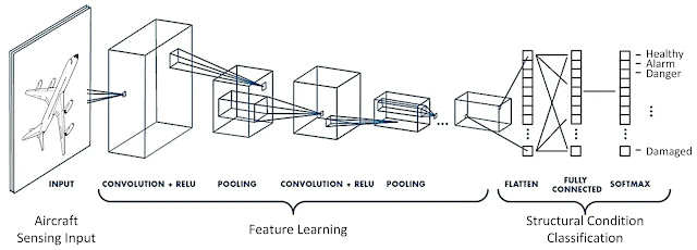
Convolutional Neural Network      CNN/ConvNet is a Deep Learning algorithm, that deals with images, it takes an input image and assigns a learnable weight and bias values, and learns to differentiate with other images . Unlike other neural networks, the preprocessing required in ConvNet is smaller. In primitive methods filters are handed engineered, with enough training and ConvNets have the ability to learn them easily. The Architecture of ConvNet is analogous to the human system of the visual cortex (connectivity pattern of neurons in the Human Brain).           Individual Neurons respond only to stimuli only the restricted region of the visual field. This is called the receptive field, and the Collection of such fields is called a visual area. What is an Image? An Image is nothing but a matrix of pixel values.  3x3 image matrix is converted into 9x1 vector.  A ConvNet is able to successfully capture the Spatial and Temporal dependencies in an image through the application of relevan

ReLU Activation  Function ReLU is the most commonly used activation function, because of its simplicity, not computationally expensive.  Advantages: It is cheap to compute. It is easy to optimize converges fast No vanishing gradient problem It is capable of outputting a true zero value allowing the activation of hidden layers in neural networks to contain one or more true zero values called Representational Sparsity Disadvantages: The downside for being zero for all negative values called dying ReLU. So if once a neuron gets negative it is unlikely for it to recover. This is called the “dying ReLU” problem If the learning rate is too high the weights may change to a value that causes the neuron to not get updated at any data point again. ReLU generally not used in RNN because they can have very large outputs so they might be expected to be far more likely to explode than units that have bounded values.

Exploding Gradient Problem What & How? The problem is that during the backpropagation traversing from the final layer to the initial layer for updating the weights in the large neural network the n derivative values are multiplied. When the derivative value is large then the gradient value exponentially increases and makes the model more unstable. This is the Exploding Gradient Problem. During the backpropagation, the large change in the weights makes the model very unstable. Solutions? Weight Initialization . Reducing the  number of layers . Gradient Clipping Weight Initialization? A careful initialization of weights should be assigned during backpropagation. This can be achieved using Random initialization. Reduce the number of layers? By reducing the number of hidden layers, the problem of exploding and vanishing gradient problem can be solved. Gradient Clipping? Gradient Clipping is a technique that tackles the problem of exploding gradient problem. The idea is very simple, tha

Tanh   Activation Function tanh Activation Function is also very similar to the Sigmoid Activation Function. But this function returns the value range(-1,1). It is Zero Centric. Advantages: It is mostly used in the output layer for binary classification. It is a good example in case when input>0, the gradient we will get all negative or positive, this will lead to an exploding or vanishing gradient problem, thus tanh will work well. Disadvantages: This lead sometimes to Saturated Gradient.