Recurrent Neural Network & LSTM
Recurrent Neural Network
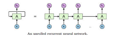
RNN is a neural network, where the output of the previous step is fed as input to the current step. The reason why the previous output is required in cases likes to predict the next word in the sentence, hence remembrance of previous words. Hence RNN has loops in them, allowing information (words) to persist.
 Here, A is a network, A gets an input X and leaves an output value h. A loop allows information to be passed from one step of the network to the next.
RNN is multiple copies of the same network, each passing the same information to the successor.
Applications of RNN
- Chat Bots
- NLP
- Translator
- Sentence completer
- Stock price Predictor, etc
The problem in Simple RNN
The problem is Long-term Dependencies. For example, consider a language model trying to predict the next word based on the previous word. If we are trying to predict the last word in "The clouds are in the sky," we don’t need any further context – it’s pretty obvious the next word is going to be "sky". In such cases, where the gap between the relevant information and the place that it’s needed is small, RNNs can learn to use past information.
But in a long context, how it works ?. For example, let us take a sentence like "My name is John, I am from Tamilnadu and I speak _____". In this, the last word can be filled with any language name. But the exact word is "Tamil". As a human, we predict the last word with the previous word "Tamilnadu". But here comes a problem of long-term dependency. Unfortunately, as that gap grows, RNNs become unable to learn to connect the information.
Vanishing & Exploding Gradient Problem
In backpropagation, during updating of weights the gradient values, using the sigmoid activation function will give rise to a vanishing gradient problem. similarly, if the weights are updated to large will rise to an exploding gradient problem.LSTM RNN
Long Short Term Memory networks (LSTM) are a special kind of RNN, capable of learning long-term dependencies. They were introduced by Hochreiter & Schmidhuber (1997). They work tremendously well on a large variety of problems, and are now widely used. LSTMs are explicitly designed to avoid the long-term dependency problem. Remembering information for long periods of time is practically their default behavior, not something they struggle to learn!
All recurrent neural networks have the form of a chain of repeating modules of neural network. In standard RNNs, this repeating module will have a very simple structure, such as a single tanh layer.
LSTMs also have this chain like structure, but the repeating module has a different structure. Instead of having a single neural network layer, there are four, interacting in a very special way.
Basically there are 4 cell and gates,
- Memory Cell
- Forget Gate
- Input Gate
- Output Gate
Memory Cell
The horizontal line passing through top is memory cell. The LSTM does have the ability to remove or add information to the cell state, carefully regulated by structures called gates. The sigmoid layer outputs numbers between "0" and "1", describing how much of each component should be let through. A value of zero means “let nothing through,” while a value of one means “let everything through!”
"+" operation is will add new context.
Forget Gate
The first step in our LSTM is to decide what information we’re going to throw away from the cell state. This decision is made by a sigmoid layer called the "forget gate layer". It looks at ht−1 and xt, and outputs a number between 0 and 1 for each number in the cell state Ct−1. A 1 represents “completely keep this” while a 0 represents “completely get rid of this.”
The next step is to decide what new information we are going to store in the cell state. This has two parts. First, a sigmoid layer called the "input gate layer" decides which values we’ll update. Next, a tanh layer creates a vector of new candidate values, C~t, that could be added to the state. In the next step, we’ll combine these two to create an update to the state.
Input Gate
It’s now time to update the old cell state, Ct−1, into the new cell state Ct. The previous steps already decided what to do, we just need to actually do it.
We multiply the old state by ft, forgetting the things we decided to forget earlier. Then we add it∗C~t. This is the new candidate values, scaled by how much we decided to update each state value.
In the case of the language model, this is where we’d actually drop the information about the old subject’s gender and add the new information, as we decided in the previous steps.
Output Gate
Finally, we need to decide what we’re going to output. This output will be based on our cell state, but will be a filtered version. First, we run a sigmoid layer which decides what parts of the cell state we’re going to output. Then, we put the cell state through tanh (to push the values to be between −1 and 1) and multiply it by the output of the sigmoid gate, so that we only output the parts we decided to.
Inspired by wonderful blog:👉 https://colah.github.io/posts/2015-08-Understanding-LSTMs/


Comments
Post a Comment